How To Use NONMAT6
1 - Setup
1.1 - System requirements
- NONMEM (NONMEM6 or NONMEM7) and MATLAB must be installed on your computer.
- MATLAB R2009b or later.
NONMAT6 doesn't require any others MATLAB toolboxes to run.
1.2 - Installation
- Download file_download NONMAT6 on your computer and unzip it.
- Open MATLAB
- Add the MACROS folder (in the NONMAT6 folder) to the MATLAB search path by selecting File → SetPath. Then click on Add Folder... and choose the MACROS folder.
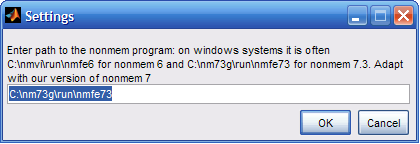
- Enter Settings in the MATLAB command window and enter path to the NONMEM program.
2 - Overview of NONMAT6
The utilisation of NONMAT6 is very easy :
- Enter SELECT (in the command window of MATLAB) and choose the control-stream file you want to analyze with NONMEM.
- Enter RUN
The RUN command launch automatically NONMEM and display a part of the NONMEM output file in the command window of MATLAB. Then you can use other commands to plot graphs and validate the model. All the commands of the toolbox are described below. You can check the full detailled toolbox commands.
| Command | Description |
|---|---|
| SELECT | Select a control-stream |
| RUN | Analyze the control-stream with NONMEM and display the results in the MATLAB command window |
| DATA | Spaghetti-plot |
| INITIAL | Search for initial values for THETA | parameters
| VAR | List the variables from NONMAT6 database |
| GOF | Goodness fit plot |
| IFIT | Individual fit plot |
| ETA | Check ETA's normality |
| ETACOV | ETA versus a covariate |
| GETA | ETA versus ETA |
| RESIDUALS | Residues |
| IDPLOT | Covariate versus ID |
| IDCONT | Contribution of individuals in the estimation of THETA |
| SE | Precision of the estimations for all the parameters |
| BOOT | Bootstrap analysis |
| NPDE | NPDE residues |
| VPPC | VPC plot |
| TEST | Test THETA=0 |
| REPORT | Show again the report after the RUN | command
| Print report + control-stream in a file | |
| SEARCH | Search observations in NONMAT6 database |
| CREATE | Create variables from NONMAT6 database in MATLAB workspace |
| GRAPH | Create a scatter-plot |
| TABLE | Create a table |
| INIVAR | RE-initialization of NONMAT6 database |
2.1 - Online help
For all the commands, a online help is available. Enter in the MATLAB command window
help command_name
2.2 - NONMAT6 database
Some commands of the toolbox use items from the data file to plot graphs. To achieve this, NONMAT6 use an internal database with the same format than the data file except that observations on doses have been deleted. More precisely, if the MDV item exists in the $INPUT field of the control-stream, then the observations with MDV=1 will be delete. If MDV doesn't exists but EVID item is, then the observations such that EVID is distinct from 0 will be delete. Finally, if neither EVID nor MDV exist then the observations with DV=0 will be deleted.
At first (just after the SELECT command), this database is made with variables in $INPUT field of the control-stream which aren't associated with DROP or SKIP. Some commands (like the RUN command ) update the database. At any time, the VAR command allows to visualize which variables are in the database. These variables are column matrix but doesn't exists in the MATLAB workspace. It is possible to create them by using the CREATE command.
2.2.1 - Database save
The database is saved when closing MATLAB. For example, if we made a RUN on the previous session, we don't have to do the same thing for the new session. We can use other commands (GOF, RESIDUALS,...) directly.
2.3 - Generalities
- Some commands open graph windows. For every window there is the string folder|name in the title bar where folder is the name of the folder which countain the control-stream and name is the name of the control-stream to remind the user the model corresponding to the figure.
- The control-stream file must NOT be in read only, it must be writable. If it's not the case, you have to change it in your computer settings.
2.4 - Display data before RUN
As we said before, after the SELECT command the database is made up with items from the control-stream $INPUT field. We can use the following commands before starting RUN (to display data for example) :
DATA, VAR, IDPLOT, GRAPH, SEARCH, CREATE, TABLE
However, you need a control-stream to do such operations. As the database is only determined by the $INPUT field, you simply have to do the simpliest control-stream as possible as for example :
$PROBLEM
$INPUT item1 item2 ...
$DATA nom
$SUBROUTINE ADVAN1
$PK
k=THETA(1)+ETA(1)
$ERROR
Y=F+EPS(1)
$ESTIMATION METHOD=0
$THETA 1
$OMEGA 1
$SIGMA 1
info_outlineOnly the commands RUN, INIVAR and BOOT (which adds NPDEvalues to the database) modify the NONMAT6 database.
3 - NONMAT6 toolbox commands
SELECT
Select a control-stream file and open it in the MATLAB editor window.
The command SELECT('demo') opens the control-stream of the theophylline available in the subfolder Example of the folder NONMAT6.
report_problemThe SELECT command must be called one time on the same control-stream. The control-stream file itself can be modified later. To be sure that the modifications are taken into account (in the database), the best procedure is to save and recall RUN which is the command (see RUN command here) that start the control-stream analysis by NONMEM.
DATA
Spaghetti-plot of DV versus TIME
The syntax DATA('expr') displays a spaghetti-plot of expr versus TIME. In this case expr can be any MATLAB expression involving database variables of NONMAT6.
Demo :
DATA('log(DV)')
RUN
This command analyzes the control-stream file with NONMEM and displays (in the MATLAB command window) some informations of the model. It also reproduces the diagnostic of the run as recorded in the NONMEM output file.
trending_flatThis file is named OUTPUT_name, where name is the name of the control-stream file and is located in the same folder as the control-stream. It is always useful to consult it.
Notes :
- Before launching NONMEM, the RUN command adds automatically the following field to the control-stream :
$COVARIANCE PRINT=E
It also adds two $TABLE fields to have a table of all variables in the $INPUT field and a table of all ETA posthoc. This edited control-stream file will be the one analyzed with NONMEM.
info_outlineYou can see this control-stream by examinating the NONMEM output file because it reproduce the last analyzed control-stream.
- In some cases, we want to launch NONMEM without including additional fields. In fact the RUN command can be declined in three ways : RUN(0), RUN(1) and RUN(2) (identical to RUN). The commands RUN(1) and RUN(2) only work in "estimation" mode i.e if an $ESTIMATION field exists in the control-stream. They are inactive if $SIMULATION or $MFSI are in the control-stream.
-
Modification of the database after RUN
The RUN command modifies the database. After the RUN command, the variables in the database are the following : - All the variables in the $INPUT field except the ones associated with DROP or SKIP.
- PRED, RES, WRES.
- All the variables in a $TABLE field without the option FILE.
- The ETA posthoc variables (ETA1, ETA2,...) for RUN or RUN(2).
| RUN(X) | Action |
|---|---|
| RUN(0) | Launch NONMEM as it is. Nothing is added to the control-stream. All the commands of the NONMAT6 toolbox are then inactive. |
| RUN(1) | Launch NONMEM in 'partial' mode, i.e with adding nothing except a $TABLE field to be able to use variables from $INPUT field. |
| RUN(2) | Same as RUN |
Demo :
Let's consider a control-stream file with two ETA, ETA(1) and ETA(2) and the following $INPUT field :
$INPUT ID AMT DV DROP=OCC
Also, let's suppose there are two $TABLE fields without the FILE option :
$TABLE IPRED IWRES
$TABLE EFF
Then the variables in the NONMAT6 database will be ID, AMT, DV, PRED, RES, WRES, IPRED, EFF, ETA1, ETA2.
info_outline The CREATE command (see CREATE command here) will create all or a part of these variables in MATLAB workspace under the same name. Each variable created is a column matrix as in the data file.
VAR
The VAR command displays the name of all the variables in the NONMAT6 database. If some variables have been renamed in the $INPUT field of the control-stream, the new name will replace the old one.
Demo 1 :
$INPUT ID TIME CONC=DV MDV
CONC will be displayed in VAR but DV won't be. For variables in a $TABLE field, names will follow NONMEM convention in output tables. NONMEM6 only chooses the 4 first letters.
Demo 2 :
If the control-stream displays :
$TABLE IPRED
The name displayed in VAR will be IPRE for NONMEM6 and IPRED for NONMEM7.
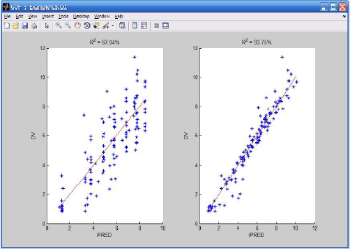
GOF
"Goodness of Fit"
Scatter-plot of DV versus PRED and DV versus IPRED (if the IPRED variable exists in the database, check Figure 2).
Two other syntaxes exist for this command :
- (a) GOF('cond')
- (b) GOF('cond1', 'color1', 'cond2', 'color2', ...)
(a) The syntax GOF('cond') does the same thing as GOF but only display observations matching the test defined by the string 'cond'. This command can be helpful if DV variable is combining observations for two types (for example med + metabolite) to verify the fit of the med observations or the metabolite. 'cond' may be with any logical expression involving logical operators and variables from NONMAT6 database. Variables name must be the one displayed in the VAR command.
(b) The syntax GOF('cond1','color1','cond2','color2',...) displays observations matching the cond1 condition with the color color1, observations matching the cond2 with the color color2 etc...
info_outlineThe colors must be MATLAB ones : red, green, blue, cyan, magenta, yellow, black, white.
Demo :
- GOF('ID==1')
- GOF('WRES>5 & TIME>1')
- GOF('TIME<5','red','TIME>=5','blue')
info_outlineUse logical operators as "&, |, ..." instead of "&&, ||, ..."
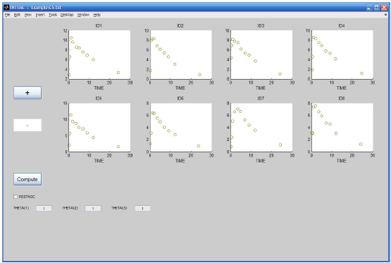
INITIAL
This command opens a graphic window (see Figure 3) to facilitate the choice of initial values (only for THETA) before applying RUN. The window displays at the top DV versus TIME individual by individual.
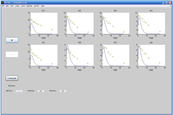
The + and - buttons allows to navigate between individuals. The compute button calculates the NONMEM predicted values (when the THETA values are the window values) and displays them on the individuals graphs (see Figure 4). The predicted values are those with all ETA equal to 0.
info_outlineIf before clicking on compute, the posthoc case is checked, then the predicted values will be those with eta posthoc. To calculate posthoc values, NONMEM use (in addition to the values of THETA) the values from the $OMEGA and $SIGMA fields of the control-stream.
info_outlineAs for GOF, INITIAL('cond') syntax do the same but only display observations matching 'cond'
Demo :
INITIAL('TYPE==1')
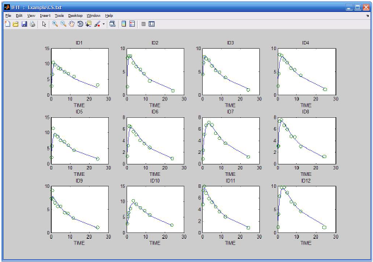
IFIT
Individual fit
Displays a graphic window (see Figure 5) to see the fit individual by individual. The + and - buttons help to progress among individuals. The curve uses IPRED values if IPRED is in the database. If some individual have been dosed in several occasions (labeled by the variable OCC in the $IMPUT field of the control-stream) then we will have a graph for each occasion. To don't take into account OCC variable put DROP=OCC in $INPUT field or rename it (recall that variables preceeded by DROP or SKIP in $INPUT aren't in the database). To save this changements, start a new RUN.
info_outlineThe IFIT('cond') syntax will only display observations matching the 'cond' condition.
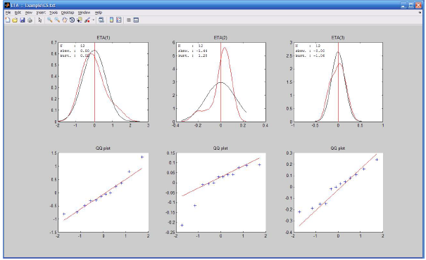
ETA
This command displays two graphs (see Figure 6) for each ETA :
- In the upper graph, the red curve is an estimation of the probability density of ETA posthoc values obtained by the kernel method. The black curve is the probability density of the normal law N(0,s²) with s² equals to OMEGA(i).
- The lower graph is a qq-plot of each ETA posthoc values.
Notes :
- A normality test for each ETA and shrinkage (ETA-shrinkage) are displayed in the MATLAB command window.
- Only the ETA with a corresponding OMEGA not fixed to 0 (in $OMEGA) are displayed.
ETACOV('expr')
Scatter-plot of post-hoc values for each ETA versus expr, which can be any MATLAB expression involving variables from NONMAT6 database.
Demo :
Suppose the variables WT and HT are in the database. Then the following syntaxes are correct :
- ETACOV('WT')
- ETACOV('log(WT)')
- ETACOV('WT./HT.^2')
In the last syntax example, the dot is due to the fact that database variables are column matrices.
GETA
Scatter-plot of ETA (posthoc) versus ETA (posthoc). This graphs are appropriated to see correlations between two ETA.
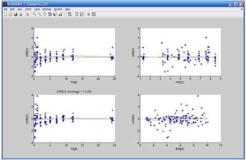
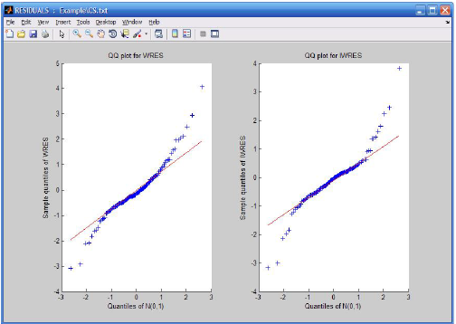
RESIDUALS
Scatter-plot of WRES vs TIME and WRES vs PRED.
Another window displays a qq-plot of WRES. If IWRES and IPRED are in the database, the command also displays a scatter-plot of IWRES vs TIME and IWRES vs IPRED (see Figure 7) and a qq-plot of IWRES (see Figure 8). Recall that IWRES is defined by the following formula :
IWRES = (DV - IPRED)/SD
with SD indicating the standard deviation.
Notes :
We also have the two following syntaxes (identical to the GOF command) :
- RESIDUALS('cond')
- RESIDUALS('cond1', 'color1', 'cond2', 'color2',...)
SE
Displays standard errors for all parameters (THETA, OMEGA and SIGMA). The RUN command only displays standard errors for THETA
IDPLOT
"Index-plot"
Scatter-plot of IWRES versus ID if IWRES is in the database, else scatter-plot of WRES versus ID.
The syntax of IDPLOT('expr') does the same thing with observations of expr which can be any MATLAB expression involving variables from NONMAT6 database.
Demo :
IDPLOT('log(WRES)')
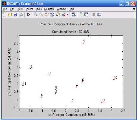
IDCONT
"Individual contribution"
This command displays a graphic window to see the influence of each individual in the estimation of THETA parameters and then allow to locate abnormal individuals.
It operates as following :
For each individual, we remove this individual from the data file and then estimate the THETA parameters by NONMEM. This process is repeated for every individual. At the end, we have (for every individual) an estimation of THETA when this individual is suppressed from the data file. Then a PCA (Principal Component Analysis) is done (see Figure 9). The results of the PCA are recorded in a text file named PCA_name (where name is the name of the control-stream file) and it is located in the same folder as the control-stream.
Notes :
There are two others syntaxes for this command :
- (a) IDCONT('file')
- (b) IDCONT('x')
(a) The IDCONT('file') command displays the graphic window again from the text file PCA_name. This command is helpful when the IDCONT command take a lot of time. For instance, it can be used to redisplay the PCA (for example after closing MATLAB) without requiring any recalculations.
(b) In this case, x is a sublist of 1:N where N is the number of individuals in the data file (1 is for the first individual of the data file, 2 for the second one etc...). The IDCONT command is similar to IDCONT(1:N). When x is distinct from 1:N, this command creates no output but only record the THETA corresponding to x in the text file PCA_name. The command IDCONT(x) allows to split IDCONT execution (if for example IDCONT execution takes too long time). We illustrate this procedure now. For example do IDCONT(1:4) to limit the execution of IDCONT after removing successively the first four individuals from the data file. Then rename PCA_name with PCA14 for example. Then call IDCONT(x) by selecting an other part of individuals, for example IDCONT(5:9). Then rename PCA_name with PCA59 and call again IDCONT(x) etc. Then merge all the PCA files in a unique file named PCA_name. Then use the command IDCONT('file').
info_outlineFor the proper functioning of IDCONT command, the field $INPUT should be preliminary to the field $DATA in the control-stream. If it's not the case, swap both fields in the control-stream.
BOOT
Bootstrap analysis of THETA estimation.
By default, 200 bootstrap files are generated. The results are displayed in the MATLAB command window. BOOT(N) command generate N bootstrap files.
NPDE
Normalised Prediction Distribution of Errors
Model testing with NPDE residuals.
By default, 200 simulations are made. If you want N simulations, enter NPDE(N). The command displays a qq-plot of the NPDE residuals and several statistics in the MATLAB command window.
info_outlineThe NPDE command adds the variable NPDEvalues (which contain NPDE residuals values) to the NONMAT6 database. See [1] and [2] for a precise definition of NPDE residuals
VPPC
Visual Post Predictive Check
By default, 100 simulations are made. The different syntaxes of this command are :
- VPPC
- VPPC(level)
- VPPC(level, rep)
- VPPC(level, rep, Nbin)
- VPPC(level, rep, Nbin, CIlevel)
level : levels vector (by default [10 50 90])
rep : number of simulated datasets (by default 100)
Nbin : bins number (by default 10)
CIlevel : confidence (by default 95%)
Demo :
- VPPC
- VPPC(50,200)
- VPPC([10,50],100,10,90)
REPORT
Re-display the report after the RUN command. The REPORT command is particularly useful after exiting MATLAB for example. It is not necessary to type RUN again (which can take some time) to see the results.
Create a text file (in the same folder as the control-stream) named RAPPORT_nom, where "nom" is the name of the control-stream file. This file is made up of two parts ; the RUN output in the first part and the control-stream in the second. This file is a good way to keep a track of the execution of a specific control-stream.
TEST
Test THETA=0 and confidence interval for each THETA. By default, the level of each confidence interval is 95%. You can change the level. Type TEST(0.90) for a confidence level of 90%.
GRAPH
Scatter-plot of expr1 versus expr2. Here, expr1 and expr2 can be any MATLAB expressions involving variables from NONMAT6 database.
The syntax GRAPH('expr1','expr2','cond') limits the display to observations matching cond condition.
Demo :
-GRAPH('log(DV)','WRES')
-GRAPH('log(DV)','log(WRES)')
-GRAPH('log(DV)','log(WRES)','ID==1')
SEARCH('cond')
Displays (in the MATLAB command window) the observation(s) of the data file matching the test defined by the string 'cond'.
Demo :
SEARCH('WRES›5 & TIME›1')
This command search in the data file, the observations such that WRES is greater than 5 and TIME greater than 1. For each observation, values corresponding to ID and TIME are displayed. To display several other variables of NONMAT6 database, just enter their name after 'cond'.
Demo :
SEARCH('WRES›5 & TIME›1','WRES','PRED')
This command will display for each observations found, the value of WRES and PRED as well as ID and TIME.
CREATE
Create variables from NONMAT6 database in MATLAB workspace.
There are two syntaxes:
- (a) CREATE
- (b) CREATE('var1','var2',...)
(a) The CREATE syntax allows to create in the MATLAB workspace all variables included in NONMAT6 database. The created variables will carry the same name.
(b) The CREATE('var1','var2,...') syntax allows only to create variables var1, var2,...
info_outlineTo check what are the variables in NONMAT6 database, use the VAR command.
Demo :
CREATE('ETA1','ETA2')
will create in MATLAB workspace two variables named ETA1 and ETA2. Each of these variables is originally a column matrix as in the data file.
Notes :
As ETA1 and ETA2 values are the same for all observations of a same individual, it can be useful to keep for ETA1 and ETA2 only one value for each individual. This can be done by a filtering variable (in this case ID) before the CREATE command by using the FILTER command. Before CREATE, enter FILTER('ID').
TABLE
Record variables from NONMAT6 database into a text file named TableExport.txt and located in the same file as the control-stream. As for CREATE, two syntaxes are possible :
- (a) TABLE
- (b) TABLE('var1','var2',...)
(a) The syntax TABLE records all variables from NONMAT6 database.
(a) The syntax TABLE('var1','var2',...) records only the variables var1, var2,...
info_outineAs for the CREATE command, FILTER can be used.
Demo :
TABLE('ID','TIME','DV','WRES')
FILTER('var')
Change the filter variable. This works only for the commands CREATE and TABLE.
In FILTER('var'), var must be a string associated to a variable of the NONMAT6 database or be equal to no. In this case, there is no filtering and variables have the same format as in the data file.
Demo :
FILTER('ID')
FILTER('no')
INIVAR
Re-initialize NONMAT6 database.
After INIVAR, the variables in the NONMAT6 database will be the variables of the $INPUT field (except variables associated with DROP or SKIP commands).
References
- [1] K.Brendel, E. Comets, C. Laffont, annd C. Lavielle. Metrics for external model evaluation with an application to the population pharmacokinetics of gliclazide. Pharmaceutical Research, 23 :2036-49, 2006.
- [2] E. Comets, K. Brendel, and F. Mentre. Model evaluation in nonlinear mixed effects models, with applications to pharmacokinetics. Journal de la Société Française de Statistique, 151 :106-28, 2010.